Dynamical System Modeling
A simulation/visualization of some a double pendulum and swinging Atwood machine accomplished with both Matplotlib and Pygame. This post is going to be a little nerdier (mathier?) than the usual ones as there hasn’t been a major or clever programming implementation. The crux of the implementation was really just solving for the system of equations, everything else was cake.
non-standard dependencies:
            matplotlib      -       pip install matplotlib
	pygame		-       pip install pygame
	scipy		-	pip install scipy
	numpy		-	pip install numpy
Inspiration
I’ve returned to school. I’m studying mechanical engineering. I’d like to be able to apply my Data Science/ Machine Learning background towards renewable energy tech. Most of them have a mechanical aspect and there can stand to be development of some of the lesser used solutions: Wave, tidal, geothermal, maybe more. Anyway, I took a class on numerical methods (using matlab 🤮). I also sweet talked my way into a graduate math class outside of my degree path using transformations to solve problems. It began with Lagrangian and Hamiltonian formulations of systems which I’ve seen before just in less detail. I decided to marry the two and write a program to visualize the motion of some systems. Enjoy!
Lagrangian vs Newtonian formulations
You may have heard of Newton’s laws: For every action there’s an equal and opposite reaction, Force = mass times acceleration. These form the foundation of the most classic analysis of a mechanical system. You draw a free body diagram, draw all forces and their reaction forces, getting as many equations as there are unknowns, then solving for those unknowns. Generally mass is known and gravity is a thing, so acceleration is what we’re interested in. We can simply integrate to get velocity and again to find position as a function of time. Now this is all you ever need to describe a system, but it can be a lot of work. As systems get more complex, this can be a daunting task. The Lagrangian is an alternative way to get the same equations.
From the way I’ve come to understand it (I could be wrong), nature tries to convert potential energy to kinetic energy in the most efficient/direct way possible. When the apocryphal apple fell from the tree to hit Newton in the head, it didn’t take a wacky path, moving left, right, or spiraling downward. It dropped straight down in the most efficient way. In the first few weeks of a calculus class, you learn to minimize a value (like surface area, velocity, whatever). By contrast, in the first day of a calculus of variations class, you learn how to minimize a function itself. This is shown to be done with the Euler-Lagrange equation. Now, there’s a function called the Lagrangian, and it’s just defined as the difference of Kinetic energy and Potential energy. (L=T-U). It’s a function, we minimize it.
Most physics students appreciate that using the principle of conservation of energy is much easier than Newton’s laws. In the same manner, we use equations of energy (Kinetic and Potential) to build the Lagrangian and then simply apply Euler-Lagrange to get our equations of motion. I’ll derive them now for the two systems in the exposition.
The systems
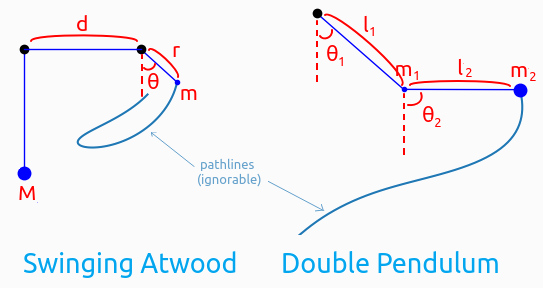 |
|---|
| The variables used in the derivations for each system shown below |
Double Pendulum
A double pendulum is probably self explanatory, it’s just a 2nd pendulum attached to the mass of a pendulum. For simplicity, I’m just considering a restricted 2D case. Kinetic energy of the system is simply the sum of the kinetic energy of both masses:
\[T = \frac{1}{2}m_1(\dot{x_1}^2+\dot{y_1}^2) + \frac{1}{2}m_2(\dot{x_2}^2+\dot{y_2}^2)\\\]I didn’t mention that these formulations can be done in any coordinates system you like. It’s pretty natural to use polar coordinates because we have masses at some distance and some angle to another point. With fixed pendulum legs, we need just two coordinates to describe the system at any point, namely the angle of the first mass from the rotation point (\(\theta_1\)) and the angle of mass 2 relative to mass 1 (\(\theta_2\)). With the length of each pendulum leg being \(l_1\) and \(l_2\). Here’s kinetic energy (after some simplification) in polar coordinates:
\[T = \frac{m_1+m_2}{2}l_1^2\dot{\theta_1^2}+\frac{m_2}{2}l_2^2\dot{\theta_1^2} + m_2l_1l_2\dot{\theta_1}\dot{\theta_2}\cos(\theta_1-\theta_2)\\\]Potential energy is easier to go straight to from polar coordinates:
\[U = -m_1gl_1\cos\theta_1 - m_2g(l_1\cos\theta_1 + l_2\cos\theta_2)\\\]We can get the Lagrangian by subtracting U from T. To apply the Euler-Lagrange equation, we must do it to each mass, giving two equations. That is we use \(\frac{d }{dt}\left(\frac{\partial L}{\partial \dot{\theta_i}}\right) = \frac{\partial L}{\partial \theta_i}\) for i = 1 and 2. With this, we have the following system of equations:
\[(m_1+m_2)l_1\ddot{\theta_1}+m+2l_2\ddot{\theta_2}\cos(\theta_1-\theta_2)+m_2l_2\dot{\theta_2^2}\sin(\theta_1-\theta_2)+(m_1+m_2)g\sin\theta_1=0\\ l_1\cos(\theta_1-\theta_2)\ddot{\theta_1}+l_2\ddot{\theta_2}-l_1\dot{\theta_1^2}\sin(\theta_1-\theta_2)+g\sin\theta_2 = 0\]I couldn’t easily, explicitly solve for \(\ddot{\theta_1}\) and \(\ddot{\theta_2}\), but I turned it into a matrix equation and solved.
\[\begin{pmatrix} (m_1+m_2)l_1 & m_2l_2\cos(\theta_1-\theta_2) \\ l_1\cos(\theta_1-\theta_2) & l_2 \end{pmatrix} \begin{pmatrix} \ddot{\theta_1}\\ \ddot{\theta_2} \end{pmatrix} = \begin{pmatrix} -(m_1+m_2)g\sin\theta_1 -m_2l_2\dot{\theta_2^2}\sin(\theta_1-\theta_2)\\ l_1\dot{\theta_1^2}\sin(\theta_1-\theta_2) - g\sin\theta_2 \end{pmatrix}\]cool? Cool. Let’s look at the next system.
Swinging Atwood Machine
The Atwood machine is just a rope that runs over two pulleys connecting two masses. A pretty lame thing to be named after. A swinging Atwood is slightly more exciting, one of the masses is allowed to swing while the other just moves up and down as usual. Here, the swinging mass is the only thing we need to describe the system, because with a fixed rope length, the other mass’s position is entirely deterministic. It’s easy to see that the Lagrangian for the system then is given as:
\(L = \frac{M}{2}\dot{r^2} + \frac{m}{2}(\dot{r^2}+r^2\dot{\theta^2}) - Mg(r+d-l)+mgr\cos\theta\) where the cool swinging mass is m, the boring mass is M, l is the length of the rope and d is the distance between the pulleys.
Now the independent coordinates are r and $\theta$. Applying Euler-Lagrange to each of these gives the following system of equations:
\[(M+m)\ddot{r} = mr\dot{\theta^2} + g(m\cos\theta-M)\\ 2r\dot r\dot\theta + r\ddot\theta^2 = -g\sin\theta\]Unlike the double pendulum, this is very easy to isolate explicitly for the acceleration terms (I’ll spare the details, it’s easy enough though)
Numerical solutions
So I used a built-in scipy solver (solve_ivp) for my first tests, it also represents the “true” solution (I’m placing more confidence in Python’s estimation. Some method called “Radau” of which I have no knowledge). But then to actually use the knowledge of the class, I converted some of my matlab (🤮) functions to python (😍). I have:
- Euler’s method
- Runga Kutta 2
- Runga Kutta 3
- Runga Kutta 4
Runga-Kutta 2 is pretty good as is; when I overlayed solutions with 3 and 4, I could hardly see a difference. Particularly when the masses came to a stop. Euler’s method sucks though (he was a brilliant dude for sure, but for his method to give nice results, the step size has to be tiny which isn’t amenable to fast calculation).
Animation
I initially animated the solutions with Matplotlib’s animation class. But when it ran, my computer fan would kick up. I also wasn’t able to get it to continuously run, I could only calculate the entire trajectory ahead of time, then run it.
In order to make the animation run continuously, I used Pygame and put a condition to recalculate the trajectory after reaching the end of the one currently being plotted. It was a natural part of the loop. It required finding a sweet spot where I don’t calculate too many terms (for fear of seeing a visible pause) and I don’t calculate too few terms in each loop (to avoid slowing down from needing to use python’s C API too frequently).
The Pygame gif below isn’t as smooth. My screencapture working at the same time led to jerky rendering. But it actually looks smoother and is definitely faster when run locally. The Matplotlib animation above was sped up to 3x speed.
Compromises
Matplotlib and Pygame individually had advantages and disadvantages, I couldn’t figure out how to get the best of both.
| MatplotLib | Pygame | |
|---|---|---|
| speed | 😢 more data = slower animation | 😊 I can set the fps |
| interactivity | 😢 None | 😊 can adjust the mass and choose solution method mid-simulation |
| overlay solutions | 😊 textbook | 😢 seizure-inducing flashes |
| ease of implementation | 😊 took a few hours | 😢 took a few days |
| other effects | 😊 pathlines shown | 😢 No pathlines |
Extra - Haunted Pendulum
Be careful when choosing your parameters, you can draw some random stuff if you’re not paying attention
c